4

Numerical solutions of the SEIR equations (describing the spreading of an epidemic disease) – or variations thereof –

  • $\dot{S} = - N$

  • $\dot{E} = + N - E/\lambda$

  • $\dot{I} = + E/\lambda - I/\delta$

  • $\dot{R} = + I/\delta$

with

  • $N = \beta I S / M$ = number of newly infected individuals

  • $\beta = $ infection rate

  • $\lambda = $ latency period

  • $\delta = $ duration of infectiosity

  • $M = S + E + I + R = $ size of the population

yield characteristic and almost symmetric peaks for the function $I(t)$ of numbers of infectious individuals. So $I(t)$ can – by a rough guess – be approximated by a Gauss curve

$$\widetilde{I}(t) = I_0\ \operatorname{exp}\Big({-\big((t-t_0)/\sigma\big)^2}\Big)$$

with $I_0$ the maximal value of $I(t)$, $I(t_0) = I_0$, and $\sigma$ such that $\widetilde{I}(0) = I(0) = 1$, i.e.

$$\sigma = t_0\ /\ \sqrt{\text{ln} I_0}$$

For different values of $\delta$, the reproduction number $R_0 = \beta\cdot\delta$, and a fixed value $\lambda = 2$ we find: enter image description here
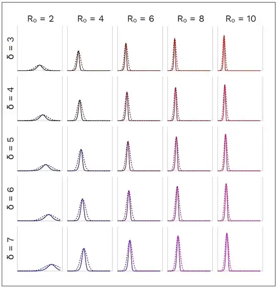
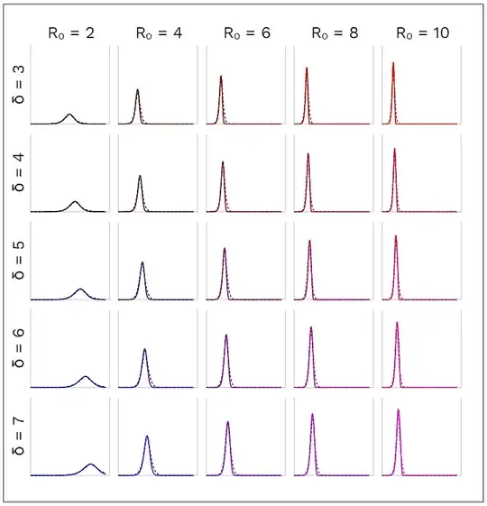
It turns out that an exponent $\sqrt{2}$ instead of $2$ yields better results, i.e.

$$\widetilde{I}(t) = I_0\ \operatorname{exp}\Big({-\big(|t-t_0|/\sigma\big)^{\sqrt{2}}}\Big)$$

enter image description here

My question is fourfold:

  1. Why is a Gauss-like curve a good approximation at all? That means: Why is $I(t)$ so symmetric?

  2. By which considerations could one come up with the exponent $\approx \sqrt{2}$?

  3. By which considerations can the asymmetry of the numerical solution $I(t)$ be understood which becomes apparent when comparing it with the symmetric approximation $\tilde{I}(t)$?

  4. Has anyone an idea how $I_0$ and $t_0$ look like as functions of $\beta,\lambda,\delta,M$?


Just to give another view on the tables above, find here all curves overlayed:
enter image description here

YCor
  • 60,149
  • If we drop the ‘E’ and stick to SIR as the simplest case, there is a variant of SIR where recovery, instead of taking place following an exponential process, occurs in constant time: see here. This variant, which can serve as an approximation to the classical case, admits an exact closed-form solution, and has a symmetric peak, so this might partially answer your question. See here for further discussion (and here for meta-discussion). – Gro-Tsen Jul 31 '20 at 12:43
  • @Gro-Tsen: Thanks for the comment and the links which I already found helpful. But please help me: What does the meta-discussion have to do with my question? Does the second-to-last link (which surely has to do with my question) refer to the article that was rejected by arXiv? – Hans-Peter Stricker Jul 31 '20 at 13:29
  • @Gro-Tsen: By the way: I can provide the same pictures as above for an SEIR model with transition from exposed to infectious and from infectious to recovered in constant times $\lambda =$ latency period and $\delta=$ duration of infectiousness (which I find less unrealistic, too).They are comparably well approximated by Gauss-like functions, so considering resp. neglecting E doesn't change so much - maybe only that there is no closed-form solution. – Hans-Peter Stricker Jul 31 '20 at 13:35
  • The meta-discussion is only mentioned to explain why the link doesn't point to the arXiv, and yes, it's the note in question (the one on hal.archives-ouvertes.fr) which was rejected thence. – Gro-Tsen Jul 31 '20 at 13:39
  • @Gro-Tsen: Did you make any progress with arXiv? Is your paper still unpublished there? – Hans-Peter Stricker Jul 31 '20 at 13:44
  • You can often get an amazingly good fit with $I_0F(t-t_0)^{-2}$ where $F(x)=(ae^{bx}+be^{-ax})/(a+b)$ with positive $a,b$, but I do not have nice approximate algebraic expressions for the parameters, just some stupid equations to solve numerically. I'll think of it a bit. – fedja Aug 01 '20 at 12:43
  • @fedja: Is your function $F(x)$ known for giving good fits in many contexts? How can these be characterized? Do you have a reference? Does $F(x)$ have a name I can google for? – Hans-Peter Stricker Aug 02 '20 at 14:26
  • @Hans-PeterStricker I posted the (partial set of) the corresponding equations. Try them and let me know what you think. Sorry for not answering earlier: had some other fish to fry. – fedja Aug 02 '20 at 23:07
  • You don't mention your initial conditions or whether your observations hold for arbitrary initial conditions. – David Ketcheson Aug 03 '20 at 11:03
  • @DavidKetcheson: I did mention - maybe not prominently enough - that I assume $\tilde{I}(t=0) = I(t=0) = 1$. – Hans-Peter Stricker Aug 03 '20 at 11:10
  • But what about S, E, and R? – David Ketcheson Aug 03 '20 at 11:29
  • @DavidKetcheson: You are right. I implicitely assumed: $S(0) = M-1$, $E(0) = 0$, $R(0) = 0$. (Better would have been to start with $E(0)=1$ and $I(0) = 0$.) – Hans-Peter Stricker Aug 03 '20 at 11:40

2 Answers2

2

Is your function F(x) known for giving good fits in many contexts? How can these be characterized?

This is too long for a comment but I'd like you to check if the fit is to your satisfaction before I elaborate. I prefer to write everything in the numerator, so my equations will be $$ \dot S=-\beta IS, \dot E=\beta IS-\lambda E, \dot I=\lambda E-\delta I\,. $$ Suppose that $I_0$ is the maximum of $I$ attained at the moment $0$ (just shift otherwise).
Then the equations I'm using (I hope I'm copyng them right) are $$ 2a^2(\beta I_0+\lambda+\delta-\mu)=\lambda\delta \beta I_0 \\ 6a^2=(\lambda+\delta-\mu)(\beta I_0-\mu) $$ Once you have solved those for $a,\mu>0$ (assume that $I_0$ is known for the moment and you just want a fitting curve rather than an independent derivation for everything), let $a_\pm=\sqrt{a^2+\frac{\mu^2}4}\mp \frac\mu 2$ (so $a_->a_+$), define $$ F_{a,\mu}(t)=I_0\left(\frac{a_-\exp(a_+t)+a_+\exp(-a_-t)}{a_-+a_+}\right)^{-2} $$ and compare it to $I(t)$. If you like the fit, we can discuss where all that nonsense came from and how to write the full system where $I_0$ will be solved for, not given. If not, I'll stop here, so let me know what you think.

The equations are algebraic of third degree, so, unless you are a big fan of Cardano's formulae, you'll have to solve them numerically. That's not hard (almost any decent iteration scheme works). The approximation is pretty good in most cases, IMHO, but it has its limitations so one can find regimes where it breaks though those are usually rather extreme. Enjoy! :-)

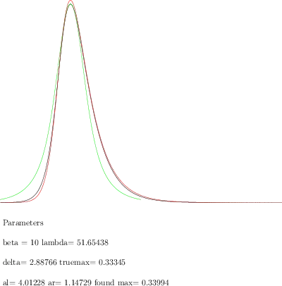
Picture 1: slightly asymmetric case

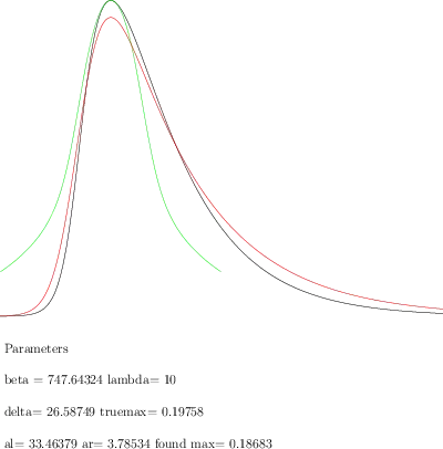
Picturee 2: Strongly asymmetric case

Two pictures, as promised. The black curve is the true trajectory, the red one is the computed trajectory (note that the height of the peak is also computed: I finally found a good third equation, so I played it honestly and didn't try to tweak the parameters beyond what my linearized equations gave directly), the green line is the best symmetric approximation you can hope for (half sum of the true trajectory and its reflection around the peak). I believe that the red line is better even without any tweaking and that the precision with which the maximum is determined is also fairly decent, but you can judge by yourself :-).

fedja
  • 59,730
  • Thanks a lot for sharing the equations. Before I start evaluating them, may I send a simplified version to you (by mail from stricker@syspedia.de), just for cross-checking (because you wrote that you're not quite sure if you copied them right)? Furthermore: Do you have a couple of plots demonstrating the goodness of fit of your approximation, ideally compared to the goodness of fit of my much simpler approximation? – Hans-Peter Stricker Aug 03 '20 at 07:42
  • 1
    @Hans-PeterStricker Yes, I have run quite a few plots. I just thought that that the surest way to evaluate a suggestion is to try it (programming takes 20 minutes to one hour) but, if you want, I'll be happy to share some pictures. Just wait a bit more until I get some free time. I double checked the equations, they seem to agree with what I have. Note that they are just linearizations of something, so if this fit is not good for some particular curve, it usually doesn't mean that the good fit does not exist, merely that you are out of the linear approximation range. – fedja Aug 03 '20 at 18:48
  • @Hans-PeterStricker OK, posted a couple of pictures. The second one is rather extreme: $R\approx 28$. Also, this is certainly not the curve of the proposed kind that fits the data best, just what the most naiive computation produces on the first run. The fit may be quite improved if you tweak it manually, but I preferred to leave it as it was;-) – fedja Aug 04 '20 at 04:04
  • Thanks so very much. Did you try or do you plan to publish this? – Hans-Peter Stricker Aug 04 '20 at 06:36
0

From an article that user @Gro-Tsen refers to I learned - and give here as a partial answer - that for the case of a vanishing latency period $\lambda = 0$, i.e. for the classical SIR model

  • $\dot{S} = -N$
  • $\dot{I} = +N - I/\delta$
  • $\dot{R} = +I/\delta$

there is a closed formula for $I_{max}$ (i.e. the maximal value of $I(t)$) as a function of $\beta$, $\delta$, and $M$ namely

$$ I_{max} = \frac{R_0 - \log R_0 - 1}{R_0} \cdot M$$

with $R_0 = \beta\cdot\delta$. This is quite nice.