Before answering this, I need to point out that a pure uniform electric or magnetic field is not a Lorentz invariant idea: different reference frames see different combinations of $E$ and $B$ fields, so I am not sure what use a description as virtual particles would have.
At the undergraduate level: avoid QFT and virtual particles. But, if you must think of virtual particles, do so as follows:
When we scatter particles, say elastic electron proton scattering:
$$ e + p \rightarrow e + p $$
all we know are the initial and final states. Each of which contain an electron and a proton, both of which are treated as non-interacting plane-waves. What happens in between is: everything. In Feynman's path integral formulation for the scattering, we add up the amplitudes for all possible particle/field configurations to get the amplitude for the process.
Now for simple problems, like Young's double slit where there are two dominate paths: (1) the particle goes through the left slit or (2) the particle goes through the right slit, that looks like:
$$ M(x) = M_L(x) + M_R(x) $$
here $x$ is the position at the detector. When you find the probability:
$$ P(x) \propto ||M(x)||^2 = ||M_L(x)||^2 + ||M_R(x)||^2 + 2M_L(x)M_L(x) $$
$$ P(x) = P_L(x) + P_R(x) + P_{int}(x) $$
voila, you have discovered particles show in wavelike interference ($P_{int}(x) $).
However, in more complex scenarios like $ep$ scattering, the exact superposition of intermediate states is completely intractable.
Enter perturbation theory. One can expand the amplitude into an infinite power series in the fine structure constant:
$$ \alpha =\frac {e^2} {\hbar c} \approx \frac 1 {137} $$
and the leading term can be drawn:

The wiggly line shows the intermediate state. It is a configuration of the electromagnetic field that transfers energy ($\nu$) and momentum ($\vec q$):
$$ q^{\mu} = (\nu, \vec q) = p^{\mu}-p'^{\mu} = k^{\mu}-k'^{\mu} \equiv -Q^2$$
and it has polarization:
$$ \epsilon = [1 + 2\frac{|\vec q|^2}{Q^2}\tan\frac{\theta}2]^{-1}$$
and no charge (it's purely electromagnetic field). It looks like a photon. It looks so much like a photon, we call it one, albeit virtual. It's virtual because when we look at the mass, $m$, we have:
$$ m^2 = q^2 \approx 4EE'\sin^2{\frac{\theta} 2} < 0$$
where $E$ ($E'$) is the initial (final) electron energy. So the squared mass is negative: that does not make sense for a real particle.
Higher order terms may look something like:
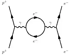
in which the virtual photon has produced an electron-positron pair with arbitrary 4-momentum running around thee loop.
Since all the terms in the perturbation series can be drawn as diagrams, and all the diagrams you can draw (with some rules) are in the perturbation series, virtual particles are an extremely handy tool for talking about processes.
For instance, if you want to discuss measuring the strange quark sea polarization in the proton via parity violating elastic scattering, you draw these 2 diagrams:

so that the parity violating signal is the interference between a photon and Z exchange.
If you want to predict the anomalous magnetic moment of the muon, which has been measured to better than 7 digits, you need to consider thousands of terms involving various intermediate states:

each of which is critical to getting the correct answer.
So virtual particles are a phenomenal tool for designing experiments or understanding processes whose exact quantitative nature are intractable, where they are not useful is in describing static field configurations.


