10

I have started to read Strogatz's Nonlinear Dynamics and Chaos and I have come across an interesting bit. He states certain damped oscillators may be modeled as having no inertia term, I.E.

$$m \ddot{x} + b \dot{x} = F(x)$$

But if $m \ddot{x}\approx 0$ (he calls this the "Inertia Term")Then it is equally valid to write

$$b \dot{x} = F(x)$$

To me, this implies that the velocity is allowed to vary depending on the spatial coordinate. However I just said a second ago that either the acceleration or the mass is negligible. So shouldn't velocity be constant?

I think what is actually going on is while a temporal change in velocity is not allowed, a spatial one still may exist. Anyways, this is still a little strange to me so does anyone know of good resources on such subjects or times when this approximation is valid?

The equation appears on page 29, concerning the impossibility of oscillations for first order ordinary differential equations.

UPDATE:

After doing a bit of reflection and dimensional analysis, I have something else to add. $m$ has dimensions of [mass], while $b$ has dimensions of $\frac{[mass]}{[time]}$. Does this mean that a viable situation when this approximation holds is for some small time scales (how small and corresponding to what, I do not know). For if some time corresponding to $b$ is small, then $b$ is large, and maybe $m \ddot{x}$ can be neglected? Can someone verify this?

user28823
  • 1,060
  • I think it means $F(t)$ and not $F(x)$. An $F(x)$ term would be spring like, a conservative force, and not an applied force. – John Alexiou Nov 10 '13 at 05:53
  • @ja72 No, Strogatz definitely meant $F(x)$. The whole book is about so-called autonomous equations, where the ODE does not explicitly depend upon $t$. $F(x)$ would be a spring like force, but it is strongly damped. – Stephen Montgomery-Smith Nov 12 '13 at 16:44
  • I am not allowed to answer the question for silly reasons. But anyway. Think about splitting the movement in two part. Around any initial starting postion x, due to the damping, the velocity approaches 0 very rapidly. Then the drag due to the potential sets in. The euqation for dragging a particle through a viscose medium is bv = F(x). – newandlost Sep 27 '17 at 10:33

5 Answers5

6

As you have noticed we cannot just solve the equation by setting $m$ to zero, this is because the term with small parameter is the only one containing the highest order derivative. In particular, Cauchy problem for the system still contains initial conditions both for, say, $x(0)$ and $\dot{x}(0)$. From the mathematical point of view such system is an example of a singular perturbation.

There are quite a lot of methods for analysis of such systems such as method of matched asymptotic expansions. Wikipedia page for it contains an example quite similar to the problem from the question.

Following this example, we apply this method here and build two approximate solutions (using notation from the question):

  • outer solution, which is valid for late times on the order of $t=O(b \cdot l / F)$ (where $l$ is the typical variation of $x$ and $F$ is the typical value of for $F(x)$) for which the governing approximate equation is $$b\, \dot{x} = F(x)$$. This is 1st order ODE, so the solution will have one integration constant.

  • inner solution, valid for small times $t=O(m/b)$. For this we rewrite the problem using rescaled time $\tau = b \cdot t/m $. The approximate equation will be $$\partial_\tau^2 x(\tau) + \partial_\tau x(\tau) =0$$. This is second order ODE, and much simpler than original system.

Then we match solutions in the overlap region, where both approximations are valid. Formally this region corresponds to dual limit: $$\lim_{\tau \to \infty} x(\tau) = \lim _{t \to 0} x (t).$$ From this equation we express one of the constant through the other two and obtain composite solution for the whole domain.

user23660
  • 5,777
2

Here's a "mathsy" explaination, but with a physical basis:

I don't know the book to which you refer but, in general, one can find which terms of an equation are dominant under given conditions through dimensional analysis. Firstly, let us imagine that there are characteristic ("distinguishing") scales that describe the amplitude, period etc. of your system so that we may write $x = \chi\hat{x}$, $t = \tau\hat{t}$ and $F=\mathcal{F}\hat{F}$, where a "hat" denotes a dimensionless variable. Then we rewrite your equation as

\begin{align} m \ddot{x} + b\dot{x} & = F(x), \\ \frac{m\chi}{\tau^2}\frac{d^2\hat{x}}{d\hat{t}^2} + \frac{b\chi}{\tau}\frac{d\hat{x}}{d\hat{t}} & = \mathcal{F}\hat{F}(\hat{x}), \\ \frac{m}{b\tau}\frac{d^2\hat{x}}{d\hat{t}^2} + \frac{d\hat{x}}{d\hat{t}} & = \frac{\mathcal{F}\tau}{b\chi}\hat{F}(\hat{x}). \\ \end{align}

Then chosing the distinguishing scale for $F$ to be $\mathcal{F} = b\chi/\tau$ we have

$$ \frac{m}{b\tau}\frac{d^2\hat{x}}{d\hat{t}^2} + \frac{d\hat{x}}{d\hat{t}} = \hat{F}(\hat{x}), $$

which is now a dimensionless equation, i.e. any pre-multiplying group (such as $m/b\tau$) has no dimensions, nor do the derivatives. If the distinguishing scales for $x$ and $t$ are carefully chosen, the derivatives (without pre-multiplying groups) are said to be of "order 1" (i.e. $d\hat{x}/d\hat{t} = O(1)$ etc.) It may now be apparent that if the group $m/b\tau \ll 1$ then the second-order derivative is of lesser importance than the other terms and can be "dropped" from the leading-order balance, leading to

$$ \frac{d\hat{x}}{d\hat{t}} = \hat{F}(x), $$

which is equivalent to your second equation. What this is telling you physically is not that the inertial term "vanishes" (i.e. we are not setting $m\ddot{x} = 0$), but rather that its numerical value is so small that it plays only a minor role in determining the dynamics of the system. In this case, the major dynamics are determined by "forcing" and "damping", or in other words the damping term dominates the inertial term in the physical balance. Other conditions will give rise to other leading-order balances which is where the "inner" and "outer" solutions mentioned by another correspondent come in.

Dai
  • 502
1

Strogatz does a nice job explaining it on page 66-69 of the book you refer to.

Write ir as a first order autonomous equation: \begin{align} \dot x &= y \\ \dot y &= \frac1m(F(x) - by) \end{align} If $by$ is much larger than $F(x)$, then $\dot y$ is very large in the negative direction. Hence y rapidly decreases. Similarly if $by$ is much smaller than $F(x)$. So after a short amount of time, $F(x) - by$ is of order $m$, which is very small. $\dot y$ is of reasonable size number, so there is no restriction on how fast $y$ can move. And substituting the first equation into all this, we get that $$ b \dot x = F(x) + O(m) .$$ By the way, I only glanced at those pages, so my argument might not do justice to Stragatz's explanation.

0

Both of the equations listed in this question are just ordinary differential equations (ODEs), which for many specific choices of $F(x)$, will be solvable analytically, using standardized techniques for solving ODEs. In the physics world, a particularly common case which often arises is $F(x) = -kx$; when this particular choice of $F(x)$ is selected, then the problem traditionally gets labeled with a special and very specific name. In that one case, it's known as the "damped harmonic oscillator" problem, and you can find many example solutions just by googling the term "damped harmonic oscillator". IMHO, I think this author provides a particularly lucid online presentation, but there are many others, including those in standard textbooks as well.

You can develop a pretty good physical intuition about the more general case, with arbitrary $F(x)$, by studying the solution for the particular case where $F(x) = -kx$, for which others have kindly already done the work ahead of you. For the standard "damped harmonic oscillator" problem, i.e., the first equation, where the inertial term is too large to be neglected, the analytic solution describing $x(t)$ will end up falling into one of three different regimes, depending upon the relative sizes of $m$, $b$ and $k$: a.) "underdamped", b.) "critically damped", or c.) "overdamped". I won't bother to explain what those terms mean here, since many other authors (e.g., the one that I provided in the link above) have already done a really good job of it. To understand what's going on with the first equation, it's helpful to read through someone else's solution to the damped harmonic oscillator problem first, and then physically plot the functional form of $x(t)$ vs. $t$ yourself, for each of the three cases. Just to be clear on what the first equation physically represents, you should be picturing a mass $m$, being dragged by a force $F(x)$ which varies with position, through a viscous medium whose thickness/viscosity/drag is governed by $b$. For the particular case of the harmonic oscillator, i.e., $F(x) = -kx$, imagine the force as being provided by a spring; i.e., the more you stretch or squeeze the spring in either direction away from its preferred resting position, the more it pushes back in the opposite direction. The relative size of the parameter $k$ encodes the sponginess/stiffness of the spring.

Anyway, the second equation, the one without the inertia term, of course has a different and simpler analytic solution for $x(t)$ than the first equation, but it's still sufficiently complicated that the solution is interesting and non-trivial. Specifically, in the harmonic oscillator case where $F(x) = -kx$, the solution will be of the form: $$x(t) = A e^{(-kt/b)}$$ (you can verify for yourself that this is indeed correct; just take the time derivative and then plug it back into the 2nd equation). Taking first and second derivatives of this expression will give you the time-dependent velocity and acceleration, and you can easily see that neither one is going to end up being constant. For the more general case, where $F(x) \neq -kx$, you will also in general get some time dependent solution for $x(t)$ which will of course be different from the harmonic oscillator solution, but in general it will still have non-zero, non-constant, time-varying velocity and acceleration.

One final point: you may ask, what physical situation does the second equation represent? In the specific case of the harmonic oscillator, where $F(x) = -kx$, you may think of it as a kind of limiting case of the overdamped oscillator already described by equation one, in which one takes the limit as $m \rightarrow 0$. Physically, the correct experimental setup to picture would be an extremely thick, viscous damping liquid, and an extremely strong, stiff spring, with a tiny mass or even no mass attached to the end of it. If you were to physically displace the spring (say, by stretching it), it would slowly deform itself back to its resting position, but once it started getting close to that equilibrium position, it would simply grind to a halt rather than overshooting past it, because the lack of an inertia term doesn't allow for overshoot.

stachyra
  • 221
0

This regime is very unintuitive and it is indeed seen very rarely in physics, though some superconducting circuits do follow a similar equation. It is complicated to deal with mathematically, as taking the limit of $m\to0$ changes the character of the ODE, but it can be done if you're careful about it. This limit is most easily understood by the principle that the particle is always travelling at the local terminal velocity.

To make this precise, consider the general equation you pose, $$ m\ddot x+b\dot x=F(x).\tag1 $$ Imagine, to begin with, that $F\equiv F_0$ is constant over some stretch of $x$. The general solution is then of the form $$x(t)=\frac {F_0}b t+x(0)-\frac mb e^{-\frac bm t}\left(\dot x(0)-\frac{F_0}b\right),$$ and it has two constants of integration, $x(0)$ and $\dot x(0)$, as corresponds to a second-order ODE. However, if the particle is very light (thought this limit is, and will be throughout, very hard to take, as $m$ carries dimensional information), then the second term becomes negligible. For one, it gets multiplied by a very small constant, so it gets smaller and smaller. Most importantly, though, the relaxation time of the exponential, $\tau=m/b$, becomes very short. This means that unless you have very sensitive time resolution, by the time you observe the particle, it will have relaxed into the terminal velocity $v_0=F_0/b$.

The same principle applies if the particle now crosses into a region that has a somewhat different force $F\equiv F_1$. The particle will take some time $\sim\tau$ to relax into the new terminal velocity, $v_1=F_1/b$, during which time the second-order character of the driving ODE will be observable, but after that all you'll see is motion at the terminal velocity.

Similarly, if $F(x)$ is some "slow" function of position, then the particle will always relax into the local terminal velocity before you've had time to realize that it does have some inertia with which to fight the 'air resistance' provided by $b$.


I know of no mechanical system where such a simplified equation could be expected to hold. If you took a mechanical particle subject to electrostatic, magnetic, gravitational, dipolar, or other such external forces, and made the mass very small, then the granularity of the medium providing the damping would become evident much before you reached this regime. Instead, you'd observe Brownian motion.

On the other hand, there is a model for superconducting circuits, and in particular for Josephson junctions in certain circumstances, that does follow this equation. This model is known as the resistively-capacitively shunted junction (RCSJ) model, and you can find OK expositions of it here and here.

Essentially, a Josephson junction is a very thin layer of insulating material in between two superconductors. The current through the junction, because of quantum mechanical effects, is given in certain regimes by $$I=I_C\sin\varphi,$$ where $I_C$ is a critical current and $\varphi$ is the phase difference between the wavefunctions of the Cooper pair condensates on either side, which grows at a rate governed by the voltage $V=\frac\hbar {q_e}\dot\varphi$ across the junction.

On the other hand, any Josephson junction still has some finite resistance (through nontrivial effects) and a very small capacitance. The simplest model that captures this is to put all three in parallel:
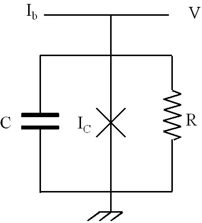
enter image description here

(Image source)

The current through the resistor is $I=V/R=\cfrac\hbar{q_eR}\dot\varphi$, whereas the current through the capacitor is $I=\dot Q=C\dot V=\cfrac{C\hbar}{q_e}\ddot\varphi$. If you hook up all three elements to a current source at current $I_0$, you'll get an equation of the form

$$I_0=I_C\sin(\varphi)+\cfrac\hbar{q_eR}\dot\varphi+\cfrac{C\hbar}{q_e}\ddot\varphi,$$

and this is of the form (1), where the force is provided by a 'tilted washboard' potential.

As it happens, the relevant limit for this equation is the overdamped case, because the "mass", $\frac{\hbar}{q_e}C$, is proportional to the capacitance, and while this is nonzero it is often (but not always) extremely tiny. Thus, you can make a mechanical analogy for this circuit, interpreting the phase $\varphi$ as the position of a 'particle', and here the inertia is often negligible.

Emilio Pisanty
  • 132,859
  • 33
  • 351
  • 666