Why do roots of polynomials tend to have absolute value close to 1?

Question

While playing around with Mathematica I noticed that most polynomials with real coefficients seem to have most complex zeroes very near the unit circle. For instance, if we plot all the roots of a polynomial of degree 300 with coefficients chosen randomly from the interval $[27, 42]$, we get something like this:

The Mathematica code to produce the picture was:

randomPoly[n_, x_, {a_, b_}] := 
  x^Range[0, n] . Table[RandomReal[{a, b}], {n + 1}];
Graphics[Point[{Re[x], Im[x]}] /. 
  NSolve[randomPoly[300, x, {27, 42}], x], Axes -> True]

If I try other intervals and other degrees, the picture is always mostly the same: almost all roots are close to the unit circle.

Question: why does this happen?

Answer 1

Let me give an informal explanation using what little I know about complex analysis.

Suppose that $p(z)=a_{0}+\dotsm+a_{n}z^{n}$ is a polynomial with random complex coefficients and suppose that $p(z)=a_{n}(z-c_{1})\cdots(z-c_{n})$. Then take note that

$$\frac{p'(z)}{p(z)}=\frac{d}{dz}\log(p(z))=\frac{d}{dz}\log(z-c_{1})+\dotsm+\log(z-c_{n})= \frac{1}{z-c_{1}}+\dotsm+\frac{1}{z-c_{n}}. $$

Now assume that $\gamma$ is a circle larger than the unit circle. Then

$$\oint_{\gamma}\frac{p'(z)}{p(z)}dz=\oint_{\gamma}\frac{na_{n}z^{n-1}+(n-1)a_{n-1}z^{n-2}+\dotsm+a_{1}}{a_{n}z^{n}+\dotsm+a_{0}}\approx\oint_{\gamma}\frac{n}{z}dz=2\pi in.$$

However, by the residue theorem,

$$\oint_{\gamma}\frac{p'(z)}{p(z)}dz=\oint_{\gamma}\frac{1}{z-c_{1}}+...+\frac{1}{z-c_{n}}dz=2\pi i|\{k\in\{1,\ldots,n\}|c_{k}\,\,\textrm{is within the contour}\,\,\gamma\}|.$$

Combining these two evaluations of the integral, we conclude that $$2\pi i n\approx 2\pi i|\{k\in\{1,\ldots,n\}|c_{k}\,\,\textrm{is within the contour}\,\,\gamma\}|.$$ Therefore there are approximately $n$ zeros of $p(z)$ within $\gamma$, so most of the zeroes of $p(z)$ are within $\gamma$, so very few zeroes can have absolute value significantly greater than $1$. By a similar argument, very few zeroes can have absolute value significantly less than $1$. We conclude that most zeroes lie near the unit circle.

$\textbf{Added Oct 11,2014}$

A modified argument can help explain why the zeroes tend to be uniformly distributed around the circle as well. Suppose that $\theta\in[0,2\pi]$ and $\gamma_{\theta}$ is the pizza slice shaped contour defined by $$\gamma_{\theta}:=\gamma_{1,\theta}+\gamma_{2,\theta}+\gamma_{3,\theta}$$ where

$$\gamma_{1,\theta}=([0,1+\epsilon]\times\{0\})$$

$$\gamma_{2,\theta}=\{re^{i\theta}|r\in[0,1+\epsilon]\}$$

$$\gamma_{3,\theta}=\cup\{e^{ix}(1+\epsilon)|x\in[0,\theta]\}.$$

Then $$\oint_{\gamma_{\theta}}\frac{p'(z)}{p(z)}dz= \oint_{\gamma_{\theta,1}}\frac{p'(z)}{p(z)}dz+\oint_{\gamma_{\theta,2}}\frac{p'(z)}{p(z)}dz+\oint_{\gamma_{\theta,3}}\frac{p'(z)}{p(z)}dz$$

$$\approx O(1)+O(1)+\oint_{\gamma_{\theta,3}}\frac{p'(z)}{p(z)}dz$$

$$\approx O(1)+O(1)+\oint_{\gamma_{\theta,3}}\frac{na_{n}z^{n-1}+(n-1)a_{n-1}z^{n-2}+\dotsm+a_{1}}{a_{n}z^{n}+\dotsm+a_{0}}dz $$

$$\approx O(1)+O(1)+\oint_{\gamma_{\theta,3}}\frac{n}{z}dz\approx n i\theta$$.

Therefore, there should be approximately $\frac{i\theta}{2\pi}$ zeroes inside the pizza slice $\gamma_{\theta}$.

Answer 2

A complete derivation can be found in the classical paper of Shepp and Vanderbei:

Larry A. Shepp and Robert J. Vanderbei: The complex zeros of random polynomials, Trans. Amer. Math. Soc. 347 (1995), 4365-4384

But the heuristic explanation is that for small modulus the higher order terms contribute very little to the polynomials, and so can be thrown away (so the polynomial can be viewed as one of much lower degree, so has not so many roots), and for large modulus, one can use the same reasoning with $z\rightarrow 1/z.$

EDIT

For a general distribution of coefficients, see this (underappreciated, in my opinion, paper): Distribution of roots of random real generalized polynomials

Answer 3

I think the following geometric argument is interesting and maybe sufficient to answer "why" at an intuitive level (?).

When we take the powers of $x$ in the complex plane, the absolute value scales geometrically ($|x^n| =|x|^n$) and the argument (angle with the x-axis) scales linearly ($\arg x^n = n \arg x$). So the powers of $x$ look like this:

If $x$ is a root of our random polynomial $$ p(x) = a_nx^n + \dots + a_1 x + a_0, $$ then each of these vectors (including the $x^0$ vector not drawn) is multiplied by a random coefficient, and the sum is equal to the zero vector. I'm just thinking of i.i.d. positive bounded coefficients for this response.

The key point is that this weighted sum of the vectors in any particular direction must cancel out to zero if $x$ is a root of the polynomial, yet each time $x^k$ goes "around the circle" the sizes $|x^k|$ of the vectors is geometrically larger --- unless $|x|$ is very close to $1$. Intuitively, some randomness in the coefficients will not be enough to cancel out large growth of $|x^k|$ because the vectors must sum to zero in every direction simultaneously.

For concreteness, choose the direction of the positive $x$-axis. Then the condition that $x$ be a root implies that, letting $\theta = \arg x$ be the angle of $x$ with the $x$-axis, \begin{align*} 0 &= \sum_k a_k Re(x^k) \\ &= \sum_k a_k |x|^k \cos (k \theta) . \end{align*} Heuristically, since $\cos(k \theta)$ is an oscillating term in $\theta$ and the $a_k$ are independently random, $|x|$ must be very close to one or else the large-$k$ terms "unbalance" the sum. And this condition must hold in all directions, not just the positive $x$-axis.

I have drawn the case where $|x| > 1$, but the $|x| < 1$ case is exactly the same.

(Edit: Maybe also interesting, in light of Francois' simulations, but this suggests that if the coefficients are all positive, or more likely to be positive, and the degree $k$ is relatively small, then we should see few roots with argument (angle to $x$-axis) close to $0$: In this case there is not enough oscillation to get cancellation. That is, the powers of $x$ don't go "around the cycle" and neither are they cancelled by negative coefficients.)

Answer 4

Think I will post this, the question remains popular and there are differing views on what it means; I wrote to Eric Kostlan, classmate, who has published on this sort of thing; he supported the answer by Phantom Hoover, saying " I was going to answer, but someone beat me to it" and sent an informal version later:

Eric Kostlan:

Its even easier, if you are willing to be non-rigorous. If you generate random polynomials in any of a number of "natural ways", the middle coefficients tend to grow fast. For example, one model which gives roots equi-distributed on the Riemann sphere gives the i-th coefficient a variance of (n choose i). So forcing all the coefficients to have the same variance is sort of like forcing the middle coefficients to be zero. So roughly speaking, this starts to look like x^n +- 1.

Here is one of Kostlan's papers in this area: https://www.ams.org/journals/bull/1995-32-01/S0273-0979-1995-00571-9/

Here is a different one, along the top of the page there is an option to download. https://doi.org/10.1016/0024-3795(92)90386-O

Answer 5

The following papers might be helpful:

Shmerling, E and Hochberg, K.J., Asymptotic Behavior Of Roots Of Random Polynomial Equations, Proceedings Of The American Mathematical Society, Volume 130 (2002), Number 9, Pages 2761-2770.

Erdős, P. and Turan, P., On the distribution of roots of polynomials, Ann. Math. 51 (1950), 105-119.

In particular, the Erdős-Turan paper contains the following beautiful result, which is a quantitative version of the observation that the angles of the roots of a random polynomial tend to be equidistributed on the unit circle. (The paper may well discuss the magnitudes of the roots, too, but this is the result that I know from that paper.)

Theorem (Erdos, Turan) Let $F(x)=\sum_{k=0}^d a_kx^k\in\mathbb{C}[x]$ with $a_0a_d\ne0$, and let $$ N(F;\alpha,\beta) = \#\bigl\{ \text{roots $r\in\mathbb{C}$ of $F$ with $\alpha\le\operatorname{arg}(r)\le\beta$}\bigr\}. $$ Then for all $0\le \alpha<\beta\le2\pi$, $$ \left| \frac{N(F;\alpha,\beta)}{d} - \frac{\beta-\alpha}{2\pi}\right| \le \frac{16}{\sqrt{d}} \cdot \left[ \log \left( \frac{|a_0|+\cdots+|a_d|}{\sqrt{|a_0a_d|}} \right) \right]^{1/2}. $$

Answer 6

I was a bit skeptical of some of the explanations, so I ran my own experiments to see how varying the parameters affected the distribution of zeros. Note that I was only interested in the case where coefficients are independent and identically distributed. Computations were done using PARI/GP instead of Mathematica.

I first essentially repeated Andrej's experiment, with degree 100 and sampling uniformly from the unit side square centered at the origin, with the expected result:

I then decided to sample uniformly from the unit side square with a corner at the origin and I saw something different:

To make sure I was seeing what I thought I was seeing, I reduced the degree to 10:

Of course, the reason is as tros443 explained, if we normalize $p(z) = a_nz^n + \cdots + a_1z + a_0$ to obtain a monic polynomial $\bar{p}(z) = z^n + \cdots + (a_1/a_n)z + (a_0/a_n),$ the normalized coefficients $a_i/a_n$ are independent identically distributed random variables with mean $1$, so the expected value of $\bar{p}(z)$ is $z^n + \cdots + z + 1$.

However at degree 10, sampling from the unit side square centered at the origin does not show this pattern at all:

The difference becomes clear when looking at roots of degree 1 polynomials, i.e. at the distribution of $-a_0/a_1$ in both cases:

In the case of the centered square, the distribution of $a_i/a_n$ has mean $0$, so the expected value of $\bar{p}(z)$ is $z^n$ rather than $z^n + \cdots + z + 1$. Note that the distribution is also very diffuse.

As I remarked in a comment to the question, the fact that the coefficients of $p(z)$ are independent identically distributed random variables implies that the distribution of zeros is invariant under $z \mapsto 1/z$, which is enough to guess that the roots will concentrate on the unit circle. However, to answer my own question, there is no reason to believe the distribution of zeros will be rotationally symmetric unless the distribution of the coefficients has mean 0.

Answer 7

Here's a simplistic intuitive explanation. First, consider the polynomial

$$x^n+x^{n-1}+\ldots+x^2+x+1$$

i.e. the polynomial of degree $n$ where all coefficients are $1$. Then all of its roots have absolute value equal to $1$. To see this, multiply it by $x-1$. This will add a new root (namely $1$):

$$(x-1)(x^n+x^{n-1}+\ldots+x^2+x+1)$$

This is equal to $x^{n+1}-1$. But $x^{n+1}-1$ has only roots with absolute value equal to $1$ (because $x^{n+1}=1$ implies that $1=|1|=|x^{n+1}|=|x|^{n+1}$).

Now lets move on to polynomials of the form

$$a_nx^n+a_{n-1}x^{n-1}+\ldots+a_2x^2+a_1x+a_0$$

where the $a_i$'s were randomly selected from a bounded interval with uniform probability. Then the $a_i$'s will be roughly equal, especially when $n$ is relatively large. That is, if $\bar a$ is the average of $a_i$'s, then by multiplying the polynomial by $\bar a^{-1}$ we will get a polynomial where the coefficients will tend to be close to $1$. Thus that polynomial will behave like the first polynomial.

Edit

The above explanation also gives you an idea why the roots are relatively evenly distributed across the unit circle.

Answer 8

This is NOT an answer, I just decided to look at what will happen if one turns this question backwards - i. e. if we want polynomials whose roots are randomly distributed in various senses (say, normally around zero with various standard deviations, or uniformly in a square around zero, or uniformly on $\mathbb C\mathrm P^1$ wrt standard metric of the Riemann sphere).

(And still later) ...trying to reconcile the pictures with what Will Sawin said, I've finally figured out that something is indeed wrong, and it has to do with precision. (A good additional motivation to clarify what's going on were upvotes starting to turn into downvotes :D )

When I increased precision, by replacing everywhere

RandomReal[{?,??}]

with

RandomReal[{?,??},WorkingPrecision->1000]

the outcome changed considerably. Typical pictures with coefficients now look like this (I hope this time precision artifacts do not distort the picture):

In most cases now there seems to be present what Will Sawin mentioned in his first comment (that rotating around zero the set of roots by an angle $\alpha$ results in rotating the $n$th coefficient by $n\alpha$).

I still do not understand why lower precision gave the pictures I produced before, and why there still is some symmetry present in most cases, but anyway this is what I've currently got.

One can still say that the placement of coefficients is far from random in any sense - there still is rotational symmetry, while absolute values of coefficients seem to form an "almost" log-concave unimodal sequence (ascending followed by descending):

I've decided to leave the rest of the message intact too.

(Added later)
As Will Sawin points out in a comment below, there is something suspicious about what follows; let me add the Mathematica code used to produce the pictures below (for the $\mathbb C\mathrm P^1$ version), maybe somebody will find some error...

RandomCP1Point[] := Module[{u=RandomReal[{-1,1}]}, 
    Exp[RandomReal[{0,2Pi}]I] Sqrt[1-u^2]/u
]
RandomCP1RootCoefficients[degree_] := Module[{L,x},
    L=CoefficientList[Times@@(x-Table[RandomCP1Point[],{degree}]),x];
    L/Max[Abs[L]]
]

Example:

ListPlot[Map[{Re[#],Im[#]}&,RandomCP1RootCoefficients[500]], 
    PlotRange->All, AspectRatio->Automatic
]

The results seem to be qualitatively indistinguishable, and the picture is quite interesting I think. I have no idea why do the coefficients tend to lie on a smooth curve, but the fact is that the density close to zero is higher than away from it.

Here are some typical results (roots are arbitrary, not complex conjugate pairs, hence coefficients are complex, not real; they are normalized by dividing through the overall maximum modulus).

Each picture contains all coefficients of a polynomial whose roots are randomly chosen in one of the above senses. The first four have 300 points, the last - 1000. In each case numbering of coefficients goes along the curve, with lowest and highest coefficients near the origin.

One more example of degree 1000 with labels for coefficient numbers:

Answer 9

This is barely more than a string of remarks but a bit long.

There are some great references given here. I think a specific question, in the spirit of the question, not answered by them is

"Under (some model of) random polynomials, what is the expected range of the non-real roots"

See some very minor computational results at the end.

For the (very) particular example giving the illustration (coefficients uniformly chosen from $[27,42]$) we could divide through by $34.5$ and rephrase (for that one example) the question as :

Setting all $a_i=1,$ the roots of $\sum_0^{300}a_iz^i$ are equally distributed on the unit circle (with a gap at $1$). Q: It seems to be about the same with $a_i$ uniformly distributed in $[1-0.22,1+0.22].$ Why?

I can think of things to say about that but won't as the whole point is that the phenomenon of "Very likely that roots very close to the unit circle and very nearly uniformly distributed in argument" is a very robust.

I find it believable and the heuristic convincing. How the random polynomials are chosen, and what the three instances of "very" mean is important for a more precise answer.

The article mentioned by Shepp and Vanderbei is great, but concerns random polynomials with coefficients from the normal distribution. At least in the example the coefficients are uniformly distributed on the real (or integer) interval $[27,42],$ that avoids a very small sector around the positive $x$-axis. Using real coefficients slightly favors the real axis. (There is at least one real root for $n$ odd. Something like $O(\ln{n})$ expected under certain assumptions.)

The mentioned paper by Schmerling and Hochberg seems quite satisfying, it just assumes that each coefficient $a_k$ comes from a distribution with a finite mean $\mu_k$ and standard deviation $\sigma_k$ which grow sub-exponentially (see the paper for a precise statement). One conclusion is that the proportion of the roots which have $1-\delta \lt |z| \lt 1+\delta$ goes in the limit to 1.

I suggested a specific question involving all the non-real roots. I'll report that I generated $100$ random polynomials $1+\sum_1^{99}a_kx^k+x^{100}$ with the $a_i$ uniformly distributed in $[0,1].$ There were $4$ real roots once, $2$ real roots $47$ times and no real roots the other $52$ times. The smallest value of $|z|$ seen among the non-real roots of any of the polynomials was $0.8365$ and was above $0.8967$ for $75$ of them. The maximum $|z|$ was $1.2386$ and for $75$ of them was below $1.1199.$ The reasoning for setting $a_0=1$ was that allowing $a_0$ very small may allow in one very small root. Perhaps dropping the one smallest and one largest $|z|$ would avoid the need for that.

Answer 10

It is interesting to consider deterministic sequences of polynomials, whose degree tends to infinity. I have two examples of proven asymptotics of the zeros.

• Let $\theta$ be a Pisot number, with minimal polynomial $P\in{\mathbb Z}[X]$. Assume that it is a cluster point in the set of Pisot numbers. Then there exists $A\in{\mathbb Z}[X]$ such that $|A|<|P|$ over the unit circle $\mathbb T$. Define $P_n(X)=X^nP(X)-A(X)\in{\mathbb Z}[X]$. This polynomial has only one root $\theta_n$ of modulus $\ge1$ ; it is again a Pisot number, whose limit is $\theta$. The other roots of $P_n$ tend to $\mathbb T$ and the empirical measure tends to the uniform measure of the unit circle.
• In 1992, I considered the (deterministic) sequence of polynomials $$q_r(X)=\prod_{j=0}^{r-1}(X+1+\frac{j}r)-\prod_{j=0}^{r-1}(1+\frac{j}r)$$ I proved that the roots concentrate, as $r\rightarrow+\infty$, along the transcendental curve $\Gamma$ of equation $$\left|\frac{(z+2)^{z+2}}{(z+1)^{z+1}}\right|=4.$$ The distribution density is $\frac1{2\pi}\rho(s)ds$ where $s\mapsto\gamma(s)$ is the arc-length parametrization of $\Gamma$ and $$\rho(s)=\Im\left(\gamma'(s)\log\frac{\gamma(s)+2}{\gamma(s)+1}\right)+\frac{\partial(P\circ\gamma)}{\partial s}\,$$ and $P$ is the solution of the non-homogeneous Neumann problem $\Delta P=0$ inside $\Gamma$ with $$\frac{\partial P}{\partial\nu}=\Re\left(\gamma'(s)\log\frac{\gamma(s)+2}{\gamma(s)+1}\right).$$ Notice that $\Gamma$ is quite close to a circle, although it is not exactly one.

Answer 11

I think the reason this is happening is that you're selecting your coefficients from a uniform distribution on the same interval. If you try running your experiment from the other direction -- that is, you look at the coefficients of a polynomial of degree $n$ with roots randomly selected from some interval $[a,b]$ (with expected value $m=\frac{b-a}{2}$) then you'd expect the coefficients to be about the same as the binomial coefficients of $(x-m)^n$. But then the $i^\text{th}$ coefficient has expected value ${n \choose i}m^{n-i} x^i$, which produces very different distributions for different values of $i$. The exception to this is if all your roots have magnitude close to $1$, in which case the $m^{n-i}$ part doesn't vary much and so you'd get coefficients more in line with the distribution you're picking from.

There are details I haven't worked out properly but I'm pretty sure this is the basic reason for what you're seeing.

Answer 12

The question that I will try to answer is:

Why do zeros of $\sum_{j=0}^n a_j z^j$ often accumulate on the unit circle when $a_j$ are iid but otherwise have a very general distribution?

My answer focuses on the role of the basis $\{z^j,\, j=0,\ldots, n\}$ for polynomials of degree at most $n$ and I will assume throughout that $a_j\sim N(0,1)$ are iid. The reason that zeros concentrate on $S^1$ is that the monomials $z^j$ are an orthonormal basis (just the usual Fourier basis) for $L^2(\delta_{S^1},\mathbb C),$ where $\delta_{S^1}$ is the uniform probability measure on $S^1.$ As explained below, the empirical measure of zeros of $\sum_{j=0}^n a_j z^j$ will converge to the same limit the empirical distribution of $n$ electrons that repel one another but are constrained to lie on the support of $\delta_{S^1}.$

If we consider instead the so-called $SU(2)$ ensemble: $$p_n(z)=\sum_{j=0}^n a_j \sqrt{\frac{n!}{j!(n-j)!}}~z^j$$ for $a_j\sim N(0,1),$ then then empirical measure for the zeros of $p_n$ converges almost surely to the uniform measure $\delta_{S^2}$ on the Riemann Sphere. This is a special case of Shiffman-Zelditch (Number Variance of Random Zeros on Complex Manifolds Geom. Funct. Anal. 18 (2008), 1422-1475) and Zeitouni-Zelditch (Large deviations of empirical zero point measures on Riemann surfaces, I: $g = 0$ IMRN Vol. 2010, No. 20, 3939-3992).

The reason is that the basis $\{\sqrt{\frac{n!}{j!(n-j)!}}~z^j, \, j=0,\ldots, n\}$ for polynomials of degree at most $n$ is an orthonormal basis for the $SU(2)-$invariant inner product on the space of polynomials of degree at most $n:$

$$\langle f,g\rangle=\int_{\mathbb C} \frac{f(z)\overline{g(z)}}{\left(1+|z|^2\right)^{N+2}}\frac{i}{2\pi}dz\wedge d\overline{z}.$$

The $SU(2)-$invariance of the inner product shows immediately that the covariance kernel of $p_n$ is $SU(2)-$invariant and hence so is the average distribution of zeros. There are also more refined results concerning weak almost sure convergence, CLTs for linear statistics, and large deviations due to Shiffman-Zelditch (Equilibrium Distribution of Zeros of Random Polynomials Int. Math. Res. Not. 2003, 25-49.) with generalizations by Bloom-Shiffman (Zeros of Random Polynomials on $\mathbb C^m$ Math. Res. Lett. 14 (2007), 469-479) that captures this behavior.

Their results work in all dimensions. I will state only a very special case in complex dimension $1$ since that seems most relevant here. These theorems, modulo some technical assumptions, say that suppose we have:

1. A compact smooth simply connected domain $\Omega\subseteq \mathbb C$
2. A (pluri)-subharmonic function $\phi$ on $\Omega$ with logarithmic growth at infinity
3. Any reasonable probability measure $\mu$ whose support is contained in $\Omega$
4. The measure $\mu$ and function $\phi$ satisfy the (rather weak) Bernstein-Markov condition.

Define $$p_n^{\mu,\phi}(z)=\sum_{j=0}^n a_j \phi_j(z),$$ where $a_j\sim N(0,1)$ are iid and $\phi_j$ are an orthonormal basis for the polynomials of degree at most $n$ with respect to the inner product coming from $L^2( e^{-n\phi(z)}d\mu(z),\mathbb C).$ Then the empirical distribution of zeros converges weakly almost surely to the equilibrium measure $\nu(\Omega, \mu, \phi),$ which is the unique minimizer of the weighted logarithmic energy $$E(\nu):=\int_{supp(\mu)}\int_{supp(\mu)} \log\left[|z-w| e^{-\phi(z)/2-\phi(w)/2}\right]d\nu(z)d\nu(w).$$

Put another way, the zeros of the random polynomial $p_n^{\mu, \phi}$ tend to be distributed precisely like electrons that are confined to stay on the support of $\mu$ and are subject to the external potential $e^{-\phi}.$ In this way, the orthonormal basis $\phi_j$ remembers the "geometry" of the domain $\Omega,$ the measure $\mu$ and the weight function $\phi,$ which is can be thought of as a Hermitian metric.

In the above setup, taking $\mu=\delta_{S^1}$ and $\phi=0,$ we recover the original "Kac" polynomials $\sum_{j=0}^n a_j z^j.$ Taking $\mu=\delta_{S^2}$ and $\phi=\log(1+|z|^2)$ recovers the $SU(2)$ polynomials.

Answer 13

I offer another point of view from the angle of the companion matrix of the polynomial. It may also give a very vague intuition about the observed uniformity of the distribution along the unit circle.

Consider the Jordan block $$J = \begin{bmatrix} 0 & 1 & & & \\ & 0 & 1 & &\\ & & &\ddots & 1\\ & & & & 0 \end{bmatrix}$$ which is the companion matrix of the zero-polynomial and has all its eigenvalues equal to zero.

Now consider a slight perturbation of this matrix in a single component in the last row, i.e. $$J_\delta = \begin{bmatrix} 0 & 1 & & & \\ & 0 & 1 & &\\ & & &\ddots & 1\\ & & \delta & & 0 \end{bmatrix}.$$ If this $\delta$ sits in $k$th entry of the last row, the eigenvalues of $J_\delta$ are the solutions of $$ z^{k-1}(z^{N-k+1} - \delta) = 0 $$ i.e. we have $k-1$ eigenvalues equal to zero and the others are the $(N-k+1)$th roots of unity times $\delta^{1/(N-k+1)}$. That means that a small perturbation in the last row throws a lot of eigenvalues from the origin towards the unit circle and the more left the perturbation is, the more eigenvalues leave the origin and also they move closer to the unit circle. In the extreme case of $k=1$ we have no eigenvalue zero anymore but all $N$th roots of unity times $\sqrt[N]{\delta}$ as eigenvalues.

Roughly, one may say that all perturbations in the last row tend to spread a number of eigenvalues equally distributed around a scaled unit circle. Moreover, the lower left corner is the most sensitive position.

Now it gets more shaky, but if we consider a perturbation in every entry of the last row and each is comparable in size, the perturbation in the lower left corner has the largest effect…

(Inspired from a talk by Sjøstrand on distributions of eigenvalues of small random perturbations of large Jordan blocks, see also the book "Spectra and Pseudospectra" by Trefethen and Embree.)

Answer 14

I have an answer that is, in content, similar to that of tros443, but with some additional detail. First, I have to make an assumption on the coefficients based on the nature of your "random" polynomial:

Suppose that the numbers $a_0, \dots, a_n$ are chosen uniformly from an interval $[m, M]$ where $M - m \ll m$.

Note that the roots of the polynomial

$$p(x) = \sum_{i = 0}^n a_i x^i$$

are independent of the scaling of $p$, so if we divide by $(m + M)/2$ we may replace this with the following assumption:

Let $\epsilon > 0$ and let the numbers $a_0, \dots, a_n$ be chosen uniformly from the ball $B_\epsilon(1)$ of radius $\epsilon$ around $1$.

In this formulation, it is acceptable for the coefficients to be properly complex. Now, for fixed $a_n = 1$, the transformation $T$ from roots $\{r_0, \dots, r_n\}$ to coefficients $\{a_0, \dots, a_{n - 1}\}$ is given by the elementary symmetric polynomials. We have the following property:

There exists a function $\delta \colon \mathbb{R}_{> 0} \to \mathbb{R}_{> 0}$ such that for all $\epsilon > 0$, we have $T^{-1}(B_\epsilon(1)^n) \subset B_{\delta(\epsilon)}(T^{-1}(\{1\}^n))$ and $\lim_{\epsilon \to 0} \delta(\epsilon) = 0$.

By $B_r(S)$ for a finite set $S \subset \mathbb{C}^n$, we mean the union of the $B_r(s)$ for each $s \in S$. This property follows from the invertibility of $DT_s$ for each $s \in T^{-1}(\{1\}^n)$, where the latter set contains all permutations of the set of roots of

$$c_n(x) = \sum_{i = 0}^n x^i,$$

which are of course the $(n + 1)$'th roots of unity; in particular, they are uniformly distributed around the unit circle. They are also distinct for each $n$, so $DT_s$ is indeed invertible for each $s$ above. (Proof: the columns of $DT_s$ are the coefficients of the $c_n(x)/(x - \zeta_i)$, where the $\zeta_i$ are the $(n + 1)$'th roots of unity, and these are linearly independent polynomials since the roots are distinct.)

The above observation then says that "roots of a polynomial whose coefficients are randomly chosen near 1, will be near the roots of unity". Here, of course, the second "near" is a relative term depending on the leading coefficient and the quantification of the first "near", but it does reproduce your observations that not only are the roots approximately on the circle, but they are, actually, approximately uniform on the circle.

Answer 15

One can explore things visually/experimentally and make good discoveries, Theory is needed to justify them. Here, however, are more experiments and speculation. This is somewhat the same thing looked at in different ways, but I think each adds something.

We see that if the (real) coefficients of $p(x)=\sum_0^n a_ix^i$ are drawn randomly from a positive interval then we can normalize to get the same roots with coefficients from $[1-\delta,1+\delta]$ and if $n$ is large enough and $\delta$ small enough relative to each other (whatever that means) the roots will be near the unit circle and almost equally distributed.

---

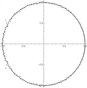
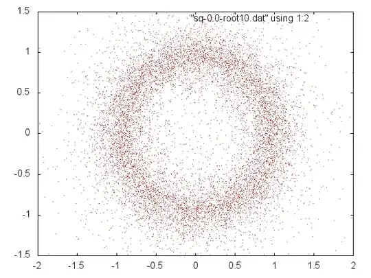
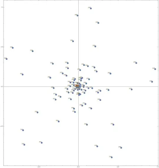
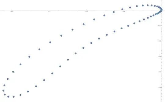
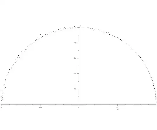
Optional example for illustration and checking: The polynomial $\sum_0^{299}z^n$ has roots $z_m=r_me^{i\theta_m}$ for $r_m=1$ and $\theta_m=\frac{2\pi m}{300}$ $1 \le m \le 299.$ I generated a single random polynomial $f(x)=1+\sum_1^{298} a_n x^x+x^{299}$ with the $a_i$ random and uniformly selected from $[0.8,1.2].$ The $299$ roots (actually, half of them) are shown below. Much can be seen but specifically: The roots, in order of increasing argument, are $r_me^{i \theta_m}$ where in all cases $0.978 \lt r_m \lt 1.036$ and $300|\theta_m-{2\pi m}| \lt 0.78.$ Here are the most extreme deviations in argument (in the upper half): $[123, -.7783]$, $[73, .7107]$, $[61, -.7036]$, $[100, -.5640]$, $[56, .5493]$, $[67, -.5482]$, $[102, -.5382]$, $[72, .5213]$, $[117, .5156]$, $[97, .5099]$, $[43, .4866]$, $[86, .4827]$, $[87, -.4749]$

---

Before going on:

• better to say the unit circle except the neighborhood of $1$. Though we could fix that by multiplying through by $x-1$ and discussing polynomials $x^{n+1}+\sum_1^{n}a_ix^i+a_0$ with $a_0$ as before but the $a_i$ in $[-2\delta,2\delta]$ (but denser near $0$.) Then the roots really are almost equally distributed.
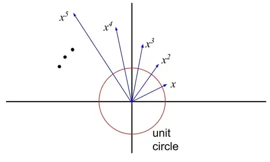
• maybe it is better to look at complex coefficients with magnitude in $[1-\delta,1+\delta]$ or $[0,1]$ or $\{{0,1\}}$
• or real coefficients of that form or from one of the sets $\{{-1,1\}},\{{0,1\}},\{{-1,0,1\}}.$

Actually these all relate to each other. Of course small perturbations of coefficients should move roots only a bit. But does that explain how little these moved?

---

If we are allowed to cook the coefficients to really move a root it seems best to move $-1$ by picking $n$ even and make the coefficients alternately $1-\delta$ and $1+\delta.$ Then $-1$ is no longer a root, $p(-1)=(n+2)\delta.$ But $p'(-1) =\frac{n+2}{2} -\frac{n^2+n}{2}\delta$ is so large that we shouldn't have to go far. In fact calculation shows that the root is roughly $-(1+2\delta).$ More precisely, exactly $-(1+2\delta+2\delta^2\cdots)=-(1+\frac{1+\delta}{1-\delta})$ and the other roots seem unchanged. Of course (in hindsight) we should just factor to see that $$p(x)=((1-\delta)x+(1+\delta))\frac{x^n-1}{x^2-1}.$$

So a root can move more than $2 \delta.$ Is that tight? Seems reasonable, but I'm not going to check. We saw only a fraction of that above. For random coefficients in our model $p(-1)=\sum(a_i-1)(-1)^i$, the sum of $n+1$ values uniformly drawn from $[-\delta,\delta]$ so not that large in relation to $p'(-1)$ . So an actual root is likely not far away at all. As far as it goes, that reasoning is valid for any of the other roots of $\sum x^i$. The root $-1$ is special, but only because we are using real positive coefficients. Arbitrary coefficient near the unit circle should resolve that.

---

If the cyclotomic roots don't move "much" then they can't end up "too close" together. But perhaps it is also good to just consider if roots (want to be) separated from each other. We could try to add a new root very near an old one or move two roots until they touch or are near. I'll leave it to you to check that, if the other roots are fixed, we get coefficients almost as large as $2.$ Can one do better moving all the roots?

---

What is the effect of each coefficient? If we change just one interior coefficient $a_k$ to something extremely huge, then there will be seen to be about $n-k$ "big" roots near equally spaced on the circle of radius $a_k^{1/(n-k)}$ and about $k$ "small" roots near the circle of radius $a_k^{-1/k}.$ We can see why. Also, for $k$ not too near either extreme, and $a_k$ merely kind of huge, we would still have all those roots quite close to the unit circle. It is far from obvious how that carries over allowing all the coefficients moving a moderate amount (randomly). Perhaps it could be said that, as long as things like $(\frac{a_{n-k}}{a_n})^{1/k}$ and $(\frac{a_k}{a_0})^{-1/k}$ are all near $1$, there should be many pullings and pushings, none very large, that usually cancel out. That is very vague and unsupported but it works for me as a motivation. With the right deliberate choices we could shove a particular root or small set of roots. That actually seems like the case above for $x=-1.$

---

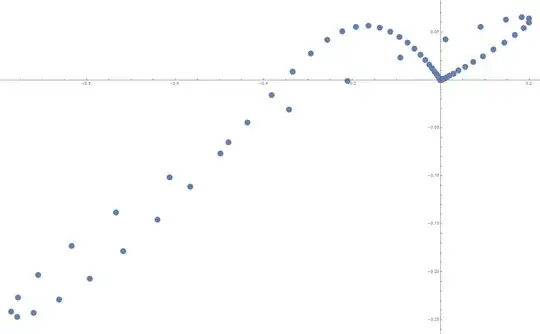
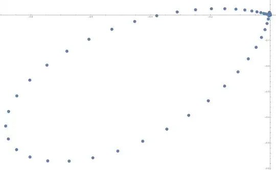
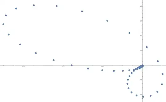
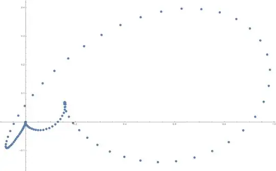
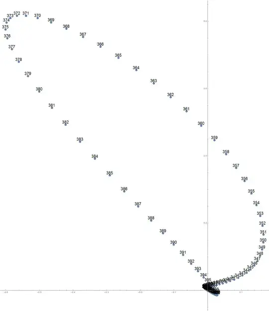
Here is an idea in perhaps more detail than it deserves. If we trace $q(x)=\frac{x^{n+1}-1}{x-1}$ as $x$ moves around the unit circle, we get a path not too hard to describe that touches the origin at the roots and then goes somewhat far away until coming back for the next one. When we perturb the coefficients and look at the position $p(x)$ on the new path, it will differ from the position on the old path by $\sum (a_i-1)x^i$ where these coefficients are random and distributed in $[-\delta,\delta]$ so the $x$ that were (near) roots of $q(x)$ will (usually) be near roots of $p(x)$ and those with $|q(x)|$ not that close to $0$ will? have the same true. It is possible to cook things to get a big deviation in one or a few places but unlikely to happen by random.

Answer 16

Old interesting question with many excellent answers. Posting this since I didn't see mentioned:

To gain intuition, you can also ask the reverse question: what needs to happen to get many large roots (e.g. norm >2) (or very small roots e.g. norm <.5, but not both)?

Assume that the coefficient for the largest power is fixed to be 1.

Assume that you have many large roots but not many small roots. Their product would be a very large number. You are bounding the coefficients to a range that is relatively very small.

What if we have both many large and many small roots? e.g. $(x-2i \cos(\theta)-2\sin(\theta))^{100}(x-.5i \cos(\rho)-.5\sin(\rho))^{100}$

First, to get real coefficients we need $100 \theta + 100 \rho\in Z$. Not a very likely event. We would also need similar conditions on $\rho$ and their relationship. Looking at the middle coefficients, these would need to cancel each other out, and the only way that can happen is if they are roughly the roots of the same number, which means the norm of the roots can not be very far from each other.