Warning: long answer ahead. To see pictures, scroll down.
A free field is just a cavity with infinitely large boundaries, right?
Right. This is how it's constructed: take a finite cavity with periodic boundary conditions, and then let its size tend to infinity.
I have also heard from many sources, including colleagues, that you can see the field as composed of a collection of harmonic oscillators separated in space.
No, the oscillators here represent eigenmodes of the field, which live in the reciprocal space—the space of wave vectors.
That would seem to imply that for each frequency, there is only one harmonic oscillator.
Not quite: for each frequency there's an infinite number of wavevectors. And for each wave vector there is one harmonic oscillator.
What is the best way to visually interpret this?
It's easier to start from simpler fields, rather than electromagnetic: in particular, in a discrete and finite medium. A good example of such a medium is a lattice of point masses connected by springs. This medium can transmit waves, and the Schrödinger's equation for such a medium is exactly solvable.
A finite chain of point masses as a model of a scalar field
$$\newcommand{\tran}{^{\mkern-1.5mu\mathsf{T}}}$$
Consider several point particles of mass $m$ connected by Hookean springs. Let one end of this chain be attached by a spring to a wall (the second end remaining free), so that all the eigenmodes of this system were standing waves, rather than running waves (this will simplify visualization a bit).

The potential energy of this system will look like
$$V(x_1,x_2,\dots,x_N)=\frac{m\omega^2}2\left(x_1^2+\sum_{n=2}^N (x_n-x_{n-1})^2\right),\tag1$$
where $N$ is number of particles, and $x_n$ is displacement of $n$th particle from its equilibrium position.
Let's denote the vector of all displacements as $\mathbf{x}$:
$$\mathbf{x}=\begin{pmatrix}
x_1\\
x_2\\
\cdots\\
x_N
\end{pmatrix}.\tag2$$
The classical equation of motion will then be
$$\frac1{\omega^2}\frac{d^2}{dt^2}\mathbf{x}=M\mathbf{x},\tag3$$
where
$$M=\begin{pmatrix}
-2 & 1 & 0 & 0 & \cdots &\cdots& 0 \\
1 & -2 & 1 & 0 & & & \vdots\\
0 & 1 & -2 & 1 & & & \vdots\\
0 & 0 & 1 & -2 & & & \vdots\\
\vdots & & & & \ddots & & \vdots\\
\vdots & & & & & -2 & 1 \\
0 &\dots&\dots&\dots& \dots & 1 & -1 \\
\end{pmatrix}\tag4$$
Notice how this matrix resembles the 1D Laplacian matrix from finite differences method. In fact, in the limit of continuous medium we'll indeed get a wave equation from $(3)$—which is isomorphic to the Klein-Gordon equation for a massless field! Due to our chosen configuration with one end being attached to a wall, and another being free, the continuous equation would have homogeneous Dirichlet boundary on one side and Neumann boundary on the other.
Substituting
$$\mathbf{x}=\mathbf A e^{i\Omega_k t},\; k\in\{1,2,\dots,N\},\tag5$$
we get the equations for eigenmodes of oscillation:
$$-\frac{\Omega_k^2}{\omega^2}\mathbf{x}=M\mathbf{x}.\tag6$$
The eigenvectors $\mathbf{\xi} _ n$ of the matrix $M$ define the axes of the hyper-ellipsoids described by $V=\mathrm{const}$. Expressed in coordinates along these axes, $V$ becomes a sum of independent oscillators—eigenmodes of the collective motion of all the particles. Namely, in this basis we'll have displacements $\mu_k$ of the modes, via
$$\mu_k=\mathbf x\tran\mathbf{\xi}_k,\tag7$$
and $V$ will get the following form:
$$V=\frac m2 \sum_{k=1}^N \Omega_k^2\mu_k^2.\tag8$$
Kinetic energy is invariant with respect to rotations in configuration space, so we don't worry about it: it'll be separable in any of these coordinates.
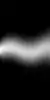
Here're the first 3 normal modes for the case $N=50$:

Quantum version of the scalar field model
Equation $(8)$ makes it very easy to solve the quantum counterpart of the problem. Namely, the Schrödinger's equation for the whole system of connected particles becomes simply a system of $N$ independent equations, one for each eigenmode.
The solution of the Schrödinger's equation,
$$-\frac{\hbar^2}{2m}\sum_{k=1}^N\partial_{x_k}^2\psi+V\psi=E\psi, \tag9$$
is the product of the well-known Hermite polynomials times Gaussians: for each mode $k$ we have
$$\psi_k(\mu_k)=\frac1{\sqrt{2^n n!}}\left(\frac{m\Omega_k}{\pi\hbar}\right)^{1/4}\exp\left(-\frac{m\Omega_k \mu_k^2}{2\hbar}\right)H_n\left(\mu_k\sqrt{\frac{m\Omega_k}{\hbar}}\right), \tag{10}$$
and the total wavefunction of the system is
$$\Psi(\mathbf{x})=\prod_{k=1}^N \psi_k(\mu_k). \tag{11}$$
Visualizations
One of the ways a quantum state can be visualized is by showing probability densities. Each mode, being a simple harmonic oscillator, will have the well-known probability distributions of the "displacement" of the mode. Visualization is trivial in these coordinates. But eigenmodes aren't something easy to intuit, so visualization in terms of them has little value.
What we'd rather have is probability densities of displacement of the particles in the chain. This is something for which we have classical intuition and also for which we have (assuming some experience in QM) intuition for the $N=1$ case, i.e. single particle.
Now, to get a probability density of displacement of a single particle in the chain we have to integrate out all particle coordinates except for ones of the particle $n$ we're interested in:
$$\rho(x_n)=\int\limits_{\mathbb{R}^{N-1}} |\Psi(\mathbf{x})|\,\mathrm{d}x_{n_1}\mathrm{d}x_{n_2}\cdots\mathrm{d}x_{n_{N-1}},\tag{12}$$
where $n_i\ne n$.
In $N\le3$ case this integration is reasonably easily doable numerically. Even in $N=4$ it's not too long to compute this integral for many points in $x_n$ for each of the particles. But the larger the number of particles, the harder this work becomes. In ref. 1 the authors claim to have used Monte-Carlo integration to obtain their probability densities. As I've tried this on my PC (using Wolfram Mathematica's NIntegrate on Intel Core i7-4765T), this direct integration approach appeared to be uselessly slow for $N=11$ even for a single value of $x_1$.
So, we need a better way to compute $(12)$. Fortunately, the wavefunction is separable in the mode coordinates $\mu_k$, so we can, instead of sampling lots of tiny probability densities $|\Psi|$ to get $\rho$, use inverse transform sampling to generate correctly-distributed points in $\mu$-space, transform the $\{\mu_k\}_k$ generated to $\{x_n\}_n$ and make $N$ histograms of $x_n$ values.
To implement inverse transform sampling, we need the following ingredients:
- CDF of the harmonic oscillator. This one is just an integral of gaussian-times-polynomial. For each excitation level $k$ there's a closed-form expression in terms of the $\operatorname{erf}$ function. If we express the wavefunction of a harmonic oscillator in terms of $s=x\sqrt\Omega$, then this integral doesn't depend on $\Omega$.
- Inverse function of the CDF. For the purposes of visualization it's sufficient to generate a table of values of the CDF for values of $s$ where the CDF is very small to where the CDF is very close to 1, and linearly interpolate between the pairs $(\mathrm{cdf}, s)$.
$n$-phonon states
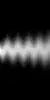
One way of visualizing a field state is by showing probability density of displacement of its particles, like it's done in ref. 1. A bit different way, similar to that used in ref. 2, is to separately take the positive and negative parts of the wavefunction, and show the "partial probabilities" of both parts e.g. in different color channels.
The following images will display the state of a 50-particle chain in both ways: gray is total probability density, red positive part, blue negative. Horizontal axis denotes the particle in the chain, while vertical axis is the displacement of the particle.
|
vacuum
(image repeated
for convenience) |
1 phonon |
5 phonons |
10 phonons |
| mode 1 |
 |
 |
 |
 |
| mode 3 |
|
 |
 |
 |
| mode 10 |
|
 |
 |
 |
|
|
1 phonon in mode 1,
4 phonons in mode 3 |
 |
10 phonons in mode 1,
1 phonon in mode 2 |
 |
10 phonons in mode 1,
1 phonon in mode 9 |
 |
One other way of visualization of stationary states is by simulating repeated measurements of the field configuration. In this case we'll see the most probable field configurations directly. This is similar to the approach in ref. 2, but instead of showing the configuration with opacity weighted by probability, we sample the configurations with its probability. Below is the visualization of the state with 15 phonons in mode 3.

Coherent states
From the previous section showing $n$-phonon states we might have concluded that for a quantum field, what's quantized is the field amplitude. This is partially right: each eigenstate has a global maximum of the probability density at a particular field amplitude, and adding phonons increases this maximum amplitude. It's similar to the amplitude of the simple harmonic oscillator, whose highest maxima also jump farther from equilibrium position as you excite it to higher energy levels.
But in fact, the most classical-like states, called coherent states, can change their amplitudes continuously. This is because their maximum is defined by the distribution of weights of the eigenstates in the superposition. This distribution can change its expected value smoothly, and so will the maximum of the probability density of displacement.
Coherent states of a field can be visualized just as easily as eigenstates, because the superposition here is taken over a single mode, which retains separability of the wavefunction. Namely, for a coherent state of $k$th mode with mean phonon number $\langle n\rangle=|\alpha|^2$, we have
$$\psi_k^{(\alpha)}(\mu_k)=\exp\left(-\frac{\alpha^2}2\right)\sum\limits_{n=0}^\infty \frac{\alpha^n}{\sqrt{n!}}\psi_n(\mu_n).\tag{13}$$
For ease of sampling though, we want a simpler expression, which can be found using the fact that a coherent state is an eigenstate of the annihilation operator. Solving corresponding differential equation, making sure the solution also solves Schrödinger's equation (by adding the necessary time-dependent phase) and normalizing will yield
$$\psi_k^{(\alpha)}(\mu_k)=\left(\frac{m\Omega_k}{\pi\hbar}\right)^{1/4}\exp\left(-\frac{m\Omega_k}{2\hbar} \left(x-\alpha\sqrt{\frac{2\hbar}{m\Omega_k}}\cos(\Omega_k t)\right)^2\right)\times\\
\times\exp\left(-i\left(\alpha x\sqrt{\frac{2m\Omega_k}\hbar}\sin(\Omega_k t)+\frac{\Omega_k t}2-\frac{\alpha^2}2\sin(2\Omega_k t)\right)\right).\tag{14}$$
Coherent states' evolution in time is non-trivial: their probability densities change. This makes the phase also evolve non-trivially, so we can't usefully show signs of the wavefunction as in ref. 2. So we'll only show probability densities now. Below are some animations of coherent states with different values of mean phonon number $\langle n\rangle$ and for different modes (frequencies are not to scale, so animations go at the same rate).
|
$\langle n\rangle=0$ |
$\langle n\rangle=0.5$ |
$\langle n\rangle=1.0$ |
$\langle n\rangle=5.0$ |
$\langle n\rangle=10.0$ |
| mode 1 |
 |
 |
 |
 |
 |
| mode 3 |
|
 |
 |
 |
 |
| mode 10 |
|
 |
 |
 |
 |
References
Scott C. Johnson, Thomas D. Gutierrez, "Visualizing the phonon wave function", 2002 Am. J. Phys. 70(3). DOI: 10.1119/1.1446858.
Helmut Linde, "A new way of visualising quantum fields", 2018 Eur. J. Phys. 39 035401. DOI: 10.1088/1361-6404/aaa032.